Bellman ford algorithm | Bellman ford algorithm in daa | Bellman ford algorithm shortest path

The Bellman-Ford Algorithm is used to find the shortest path from a single source vertex to all other vertices in a weighted graph. Unlike Dijkstra’s algorithm, Bellman-Ford works with graphs that contain negative weight edges and detects negative weight cycles.

Key Features of Bellman-Ford

✅ Works with negative weight edges
✅ Detects negative weight cycles
❌ Slower than Dijkstra’s algorithm
❌ Doesn’t work with undirected negative weight cycles

Time Complexity

• O(V * E) (V = vertices, E = edges)
• Slower than Dijkstra but handles negative weights.

Algorithm Steps:

1. Initialize:
   • Set the distance to the source node as 0.
   • Set the distance to all other nodes as ∞ (infinity).
2. Relax All Edges (V-1 times):
   • Repeat (V – 1) times (where V is the number of vertices).
   • For each edge (u → v) with weight w, update the distance: if distance(u)+w<distance(v), then update: distance(v)=distance(u)+w
3. Check for Negative Weight Cycles:
   • Run the algorithm one more time.
   • If any distance is updated again, it means a negative weight cycle exists in the graph.

Example 1:

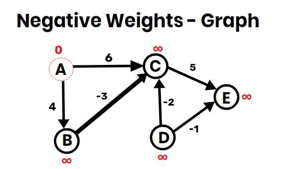
Consider the following graph where the source vertex is A:

Edge	Weight
(A, B)	4
(A, C)	6
(B, C)	-3
(C, E)	5
(D, C)	-2
(D, E)	-1

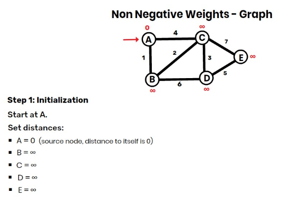
Step 1: Initialize Distances

• Source = A
• Initial Distances:
  • A = 0
  • B = ∞
  • C = ∞
  • D = ∞
  • E = ∞

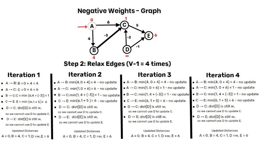
Step 2: Relax Edges (V-1 = 4 times)

• Iteration 1:
  • A → B: B = min(∞, 0 + 4) = 4 ✅
  • A → C: C = min(∞, 0 + 6) = 6 ✅
  • B → C: C = min(6, 4 + (-3)) = 1 ✅
  • C → E: E = min(∞, 1 + 5) = 6 ✅
  • D → C: dist[D] is still ∞, so we cannot use D to update C ❌
  • D → E: dist[D] is still ∞, so we cannot use D to update E ❌

Updated Distances: A = 0, B = 4, C = 1, D = ∞, E = 6

• Iteration 2:
  • A → B: B = min(∞, 0 + 4) = 4 – no update ❌
  • A → C: C = min(∞, 0 + 6) = 6 – no update ❌
  • B → C: C = min(6, 4 + (-3)) = 1 – no update ❌
  • C → E: E = min(∞, 1 + 5) = 6 – no update ❌
  • D → C: dist[D] is still ∞, so we cannot use D to update C ❌
  • D → E: dist[D] is still ∞, so we cannot use D to update E ❌

Updated Distances: A = 0, B = 4, C = 1, D = ∞, E = 6

• Iteration 3 and 4:
  • No further updates → Algorithm stops early.

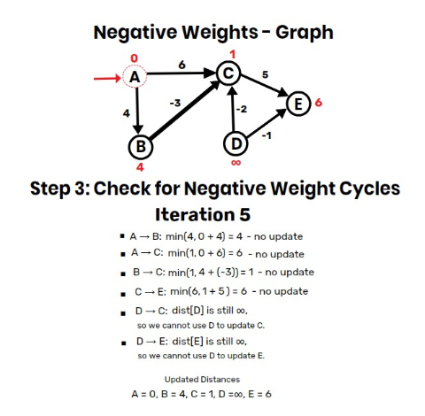
Step 3: Check for Negative Weight Cycles

• If any distance updates after one more relaxation, a negative weight cycle exists.
• Here, no further updates → No negative cycle.

Let’s now work through an example where a negative weight cycle exists and see how the Bellman-Ford algorithm detects it.

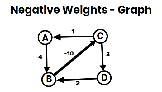
Example 2:

Consider the following graph:

Edge	Weight
(A, B)	4
(B, C)	-10
(C, D)	3
(D, B)	2
(C, A)	1

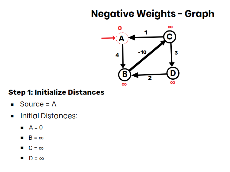
Step 1: Initialize Distances

• Source = A
• Initial Distances:
  • A = 0
  • B = ∞
  • C = ∞
  • D = ∞

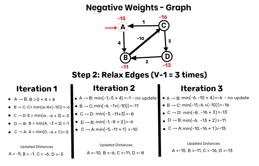
Step 2: Relax Edges (V-1 = 3 times)

• Iteration 1:
  • A → B: B = 0 + 4 = 4 ✅
  • B → C: C = min(∞, 4+(-10)) = -6 ✅
  • C → D: D = min(∞, -6+3)) = -3 ✅
  • D → B: B = min(4, -3+2) = -1 ✅
  • C → A: A = min(0, -6+1) = -5 ✅

Updated Distances: A = -5, B = -1, C = -6, D = -3

• Iteration 2:
  • A → B: B = min(-1, -5+4) = -1 – no update ❌
  • B → C: C = min(-6, -1+(-10)) = -11 ✅
  • C → D: D = min(-3, -11+3)) = -8 ✅
  • D → B: B = min(-1, -8+2) = -6 ✅
  • C → A: A = min(-5, -11+1) = -10 ✅

Updated Distances: A = -10, B = -6, C = -11, D = -8

• Iteration 3:
  • A → B: B = min(-6, -10+4) = -6 – no update ❌
  • B → C: C = min(-11, -6+(-10)) = -16 ✅
  • C → D: D = min(-8, -16+3)) = -13 ✅
  • D → B: B = min(-6, -13+2) = -11 ✅
  • C → A: A = min(-10, -16+1) = -15 ✅

Updated Distances: A = -15, B = -11, C = -16, D = -13

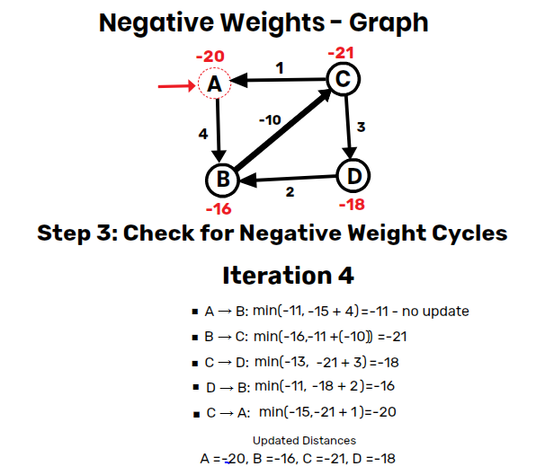
Step 3: Check for Negative Weight Cycles

• If any distance updates after one more relaxation, a negative weight cycle exists.

• Iteration 4:
  • A → B: B = min(-11, -15+4) = -11 – no update ❌
  • B → C: C = min(-16, -11+(-10)) = -21 ✅
• Since we could update C, this indicates a negative weight cycle exists, and the algorithm stops here.

Negative Weight Cycle in this Graph:

• The negative weight cycle is formed by the edges:
  • B → C → D → B with total weight: -10 + 3 + 2 = -5.